(All the Excel charts in my book are available for download, but I promised to write tutorials for a few of them. This is the first one.)
Name: Bullet charts
What it is used for: to display key performance indicators. Use them to replace speedometers if you want a more compact visual that can be stacked to better compare KPI. Also, speedometers suck.
Excel implementation: There are a few different ways to implement this chart in Excel. Jon Peltier suggests using bar charts. In this post, we will use a scatterplot.
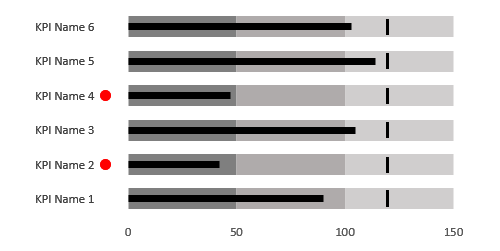
So, let’s use a KPI that can assume values between zero and 150. The cut-off points are 50 and 100 (you can have as many ranges as you like, but three is the standard number). Since I’m designing a horizontal bullet chart, all data points will have the same y value.
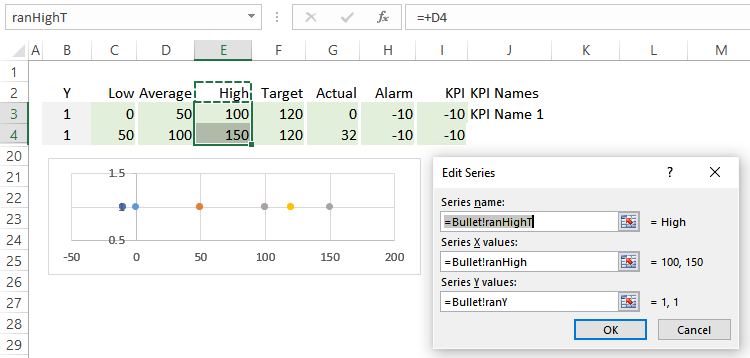
As you can see in the image above, the series High gets its data from three named ranges:
- the series name comes from cell E2 (range “ranHighT”),
- the series X value comes from cells E3:E4 (range “ranHigh”),
- and the series Y value comes from cells B3:B4 (range “ranY”).
- All series share the same y values.
Those are the background series. Now we have to add the target value and the actual value. Add them exactly as you did for the previous series. Then, we have the alarm. The alarm is not in the original specifications but, since we will need to call the reader’s attention to abnormal values, adding an alarm to the bullet chart is an elegant way to do it. In this example, there is a rule in cell H4 that returns an error if the Actual value is above the upper limit of the Low range: “=IF(G4<C4,-10,NA())”. This means that the alarm is not visible if the formula returns an error. The alarm will be displayed to the left of the chart, at value -10 (we can change this).
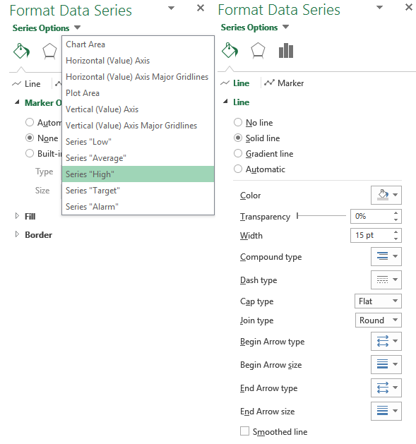
Now we have to change the Low, Average and High series. For each one, set Marker to “None”, Line width to 15 pt and Cap type to Flat.
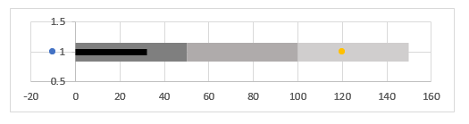
Remove marker from series Actual, change line width to 5, color to black and Cap type to Flat. Now your chart should look something like this:
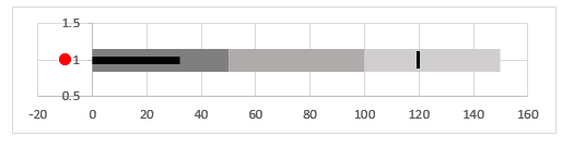
The built-in marker types don’t include a vertical line, but you can make one to use in the Target series:
- if you use Windows, open the Paint application;
- create an image sized 15 x 2 pixels;
- fill it with the color you want;
- save it;
- from the built-in types, select Image;
- choose the one you just created;
- set Marker border to No line;
- keep the Alarm marker;
- change its color to red;
- change its size to 8.
The remaining changes are more or less cosmetic:
- add the series KPI;
- remove markers and lines from the series;
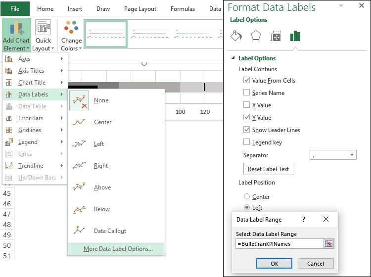
- select the KPI series and, under Design, choose Add Chart Element / Data Labels / More Data Label Options…;
- set Label Position to Left;
- check Choose Value from Cells;
- set the data range to “Bullet!ranKPINames”, the named range in column J (don’t forget the “Bullet!” part);
- uncheck “Y Value” and “Show Leader Lines”.
- remove he chart border.
You’ll have to adjust chart or plot area sizes so that the label doesn’t overlap the alarm. After these changes, the bullet chart should look like this:

I removed all gridelines and axis lines, the the labels in the vertical axis, and used a custom number format to hide negative values (add “##;;0” as a format code). The horizontal axis is set to a minimum of -50 and a maximum of 150.
Have you noticed in the first image that some of the rows are hidden? I actually defined the named ranges to go down to row 19. When you unhide these rows you’ll see five more bullet charts:
That’s it: a very simple way of making bullet charts. Was it useful? How would you improve the tutorial? Your suggestions are welcome, and let me know which chart from the book you’d like me to write about.
Here is the xls file.
And remember: clueless, one-eyed, 3D-pie loving creatures lurk in the shadows of business reports. When someone buys my book I get stronger and can join the heroes fighting these creatures.